
Welcome to the second chapter of our Modelica series. In the previous chapter, we introduced Modelica and learned how to use and simulate a model from the Modelica Standard Library. In this chapter, we will learn more about dynamic simulations and how to write equations in Modelica.
If you missed the previous chapter, you might want to read it through before starting with this one. You can find it here.
All set? Let's begin!
Dynamic simulations
In the first chapter, we worked with the graphical interface of your Modelica tool to simulate a ready-made pendulum model from the Modelica Standard Library. Only a few seconds after we pressed the simulate button, results showing the dynamic behavior of the pendulum popped up in our variable browser. You might ask yourself what goes on under the hood. How does it work? Magic?!?
The outputted behavior is due to the dynamic equations that describe each of the subcomponents of the pendulum. These equations mimic the physical behavior of the individual components. When we combine these components in a certain way, they give us the dynamic behavior of the pendulum.
In the following example, we'll have a closer look at how to write equations in Modelica.
The high-flying ball
In this example, we'll study the dynamics of tennis. To be precise, what happens when we throw a tennis ball straight up into the air at the beginning of a serve.
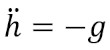
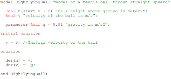
Start by creating a new model in your Modelica editor and give it an appropriate name. I'm calling mine HighFlyingBall. The first thing to model is what happens when we drop the ball from a certain height. This is described by the relation below. The variable h is the height of the ball above the ground, and g is the acceleration of gravity.
Coding in Modelica
Now, make sure that you are in the Text view of your Modelica editor. The text view is where you declare variables and write equations. Variable declarations are made at the beginning of the model, and equations are written after the equation keyword.
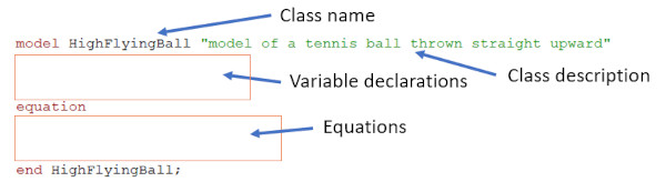
We start by declaring variables for the height, h, and the velocity, v. In Modelica, there are four default variable types: Real (floating point), Integer, Boolean, and String. Since we need our height and velocity to hold any real number, we declare them as Reals. We also add a start value to the h variable to model that we drop the ball from 1.2 meters. The acceleration of gravity, g, should also be a Real variable, but we don't need it to change during the simulation. We emphasize this by adding the prefix parameter to the declaration. We also give it a default value of 9.81 m/s².
Now we need to add some equations for the relation above. Equations in Modelica are acausal and describes relations rather than assignments, meaning that we can write them in any order and any form. Just like when writing equations on paper. Give it a try! When done, you should have something similar to this:
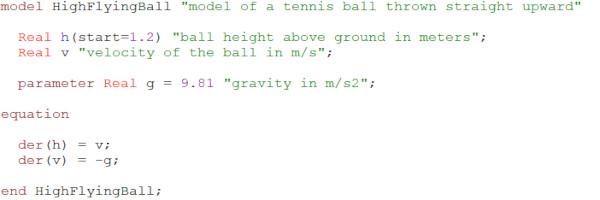
Here, we've used the der()-operator of Modelica to get the time derivatives of the variables h and v. Now, use the check functionality of your Modelica editor to check that the syntax is correct. If everything is fine, you're ready to run the simulation. Simulate for 0.5 seconds and plot the h variable.
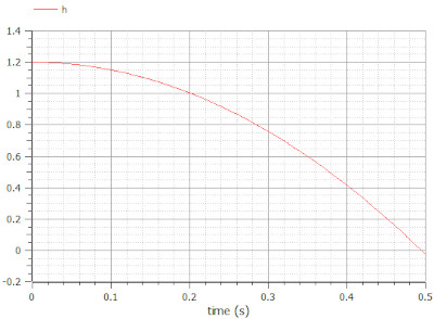
Success! The ball falls towards the ground. Just before the simulation stops, it even falls below the ground, but let's not worry about that for now.
We're almost there, but the tennis ball is still not thrown up into the air at the beginning of our simulation. We can model this by adding a positive start velocity to the v variable. We can add this start value in the same way as we did for the height, but there are other ways. This time we'll use an initial equation. Initial equations are executed at the beginning of a simulation. They're written in a separate section of a model, before or after the equation section, marked by the keyword initial equation. Add an initial equation section to your model with the initial condition v=5 m/s.
You can now check the model using the check functionality. Then simulate for 1.25 seconds and plot the height of the ball.
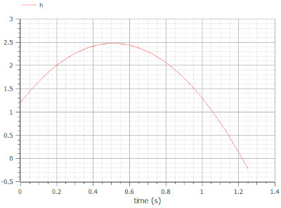
Another success! The tennis ball is thrown straight up into the air. It approaches 2.5 meters, and then it gently drops towards the ground. Now, imagine that you hit it hard with your racket.
A perfect serve! Game, Set, Match!
Modeling using the Modelica Standard Library
In the example above, you've learned how to write equations in the Text view of your Modelica editor. But in many cases, we don't need to write the equations ourselves. As seen in the pendulum example, many of the most commonly used equations are already implemented and available in the Modelica Standard Library. Does this mean that we can recreate the High-flying ball example graphically using components from the Modelica Standard Library?
To find out, we need to do some modeling. Start by creating a new model in your Modelica editor. Then go to the Diagram view. Drag and drop the following components from the Modelica Standard Library: Modelica.Mechanics.MultiBody.Parts.Body and Modelica.Mechanics.MultiBody.World. The body component models the ball, and the world component defines the gravity field.
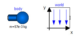
Open the parameter dialog of the body and add r_CM = {0,0,0} and m = 57e-3 kg. The latter value is the mass of a typical tennis ball. We now have a free-falling body. To model that the ball is thrown upwards from 1.2 meters, we need to modify the initial conditions for the height and velocity. This is done in the Initialization tab of the parameter dialog.
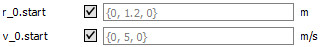
We're now good to go. Simulate for 1.25 seconds, with or without 3D animation, and plot body.r_0[2]. It is the position of the ball in the y-direction. It seems we've managed to recreate the behavior of our high-flying ball.
![Plot of the ball height, body.r_0[2], when the ball is thrown straight up into the air from 1.2 meters](/images/Blog/Modelica/ball_graphical_plot.jpg)
We've now learned how to write equations in Modelica. In the coming chapters of our Modelica series, we'll talk more about Modelica, how it works, interfaces, and applications. Check out the next chapter now!
🚀 Ready to Go Further with Modelica?
Take your modeling skills to the next level with our Modelica Introduction Course. In just two days, you'll gain hands-on experience in system modeling and simulation, perfect for engineers, innovators, and anyone ready to build smarter systems.
👉 Explore the Modelica Introduction Course »